In this post, I share my views on the Bayesian Quadrature method for policy gradient estimation. In particular, this blog is only a subset of my findings from my recent colaboration with Kamyar Azizzadenesheli (Purdue University), Mohammad Ghavamzadeh (Google Research), Anima Anandkumar (Caltech & NVIDIA), and Yisong Yue (Caltech). For full details, do check-out our Deep Bayesian Quadrature Policy Optimization paper and its accompanying resources:

PDF Slides BibTeX Code

  @article{ravi2020DBQPG,
  title={Deep Bayesian Quadrature Policy Optimization},
  author={Ravi Tej Akella and Kamyar Azizzadenesheli and Mohammad Ghavamzadeh and Anima Anandkumar and Yisong Yue},
  journal={arXiv preprint arXiv:2006.15637},
  year={2020}
  }
  

TL; DR

Bayesian Quadrature method provides a way to approximate numerical integration under a probability distribution using samples drawn from the same distribution. As it happens, policy gradient is also an intractable integral equation which is generally approximated using samples. That's pretty much it! BQ can be used for approximating PG.

But, why exactly do we need BQ-PG? : BQ-PG has several interesting properties, such as (i) a faster convergence rate over MC-PG (under mild regularity assumptions), (ii) connections to Monte-Carlo (MC) estimator, the predominant choice for PG estimation, and (iii) the explicit quantification of uncertainty in PG estimation. But even if theory does not interest you, this approach empirically offers (i) more accurate policy gradient estimates with a significantly lower variance, and (ii) a consistent imporvement in sample complexity and average return across $7$ MuJoCo benchmark environments. So the question really is “Why not BQ-PG?”.

Problem Formulation

State-Space	$s_t \in \mathcal{S}$
Action-Space	$a_t \in \mathcal{A}$
Transition Kernel	$P : \mathcal{S} \times \mathcal{A} \rightarrow \Delta_\mathcal{S}$
Reward Kernel	$r: \mathcal{S} \times \mathcal{A} \rightarrow \mathbb{R}$
Initial State Distribution	$\rho_0:\mathcal{S} \rightarrow \Delta_\mathcal{S}$
Stochastic Policy	$\pi_{\theta}: \mathcal{S} \rightarrow \Delta_\mathcal{A}$

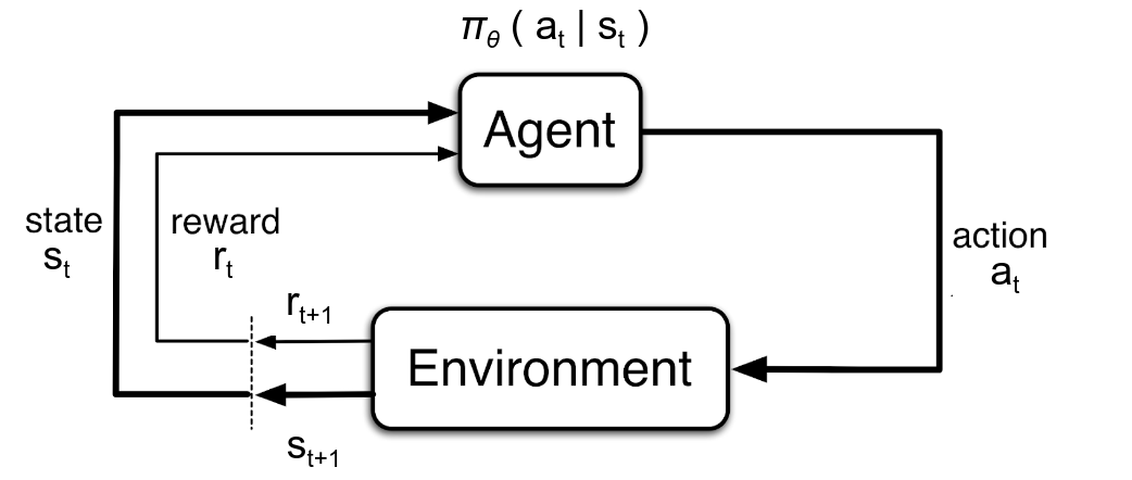
Consider a Markov decision process (MDP) $\langle\mathcal{S}, \mathcal{A}, P, r, \rho_0, \gamma\rangle$, where $\mathcal{S}$ is the state-space, $\mathcal{A}$ is the action-space, $P : \mathcal{S} \times \mathcal{A} \rightarrow \Delta_\mathcal{S}$ is the transition kernel that maps each state-action pair to a distribution over the states $\Delta_\mathcal{S}$, $r: \mathcal{S} \times \mathcal{A} \rightarrow \mathbb{R}$ is the reward kernel, $\rho_0:\mathcal{S} \rightarrow \Delta_\mathcal{S}$ is the initial state distribution, and $\gamma \in [0,1)$ is the discount factor. $\pi_{\theta}: \mathcal{S} \rightarrow \Delta_\mathcal{A}$ denotes a stochastic parameterized policy with parameters $\theta\in\Theta$. The MDP controlled by the policy $\pi_{\theta}$ induces a Markov chain over state-action pairs $z = (s,a) \in \mathcal{Z} = \mathcal{S} \times \mathcal{A}$, with an initial density $\rho^{\pi_{\theta}}_0(z_0) = \pi_{\theta}(a_0|s_0) \rho_0(s_0)$ and a transition probability distribution $P^{\pi_{\theta}}(z_t|z_{t-1}) = \pi_{\theta}(a_t|s_t) P(s_t|z_{t-1})$. The discounted state-action visitation frequency $\rho^{\pi_{\theta}}$ is defined as: \begin{equation} \label{eqn:state_visitation} P^{\pi_{\theta}}_t(z_t) = \int_{\mathcal{Z}^t} dz_0 ... dz_{t-1} P^{\pi_{\theta}}_0(z_0) \prod_{\tau=1}^t P^{\pi_{\theta}}(z_\tau|z_{\tau-1}), \qquad \rho^{\pi_{\theta}}(z) = \sum_{t=0}^{\infty} \gamma^t P^{\pi_{\theta}}_t(z). \end{equation} The action-value function $Q_{\pi_{\theta}} (z)$ denotes the expected sum of (discounted) rewards along a trajectory starting from $z = (s,a)$ and jointly-controlled by the agent's policy $\pi_{\theta}$ (known) and MDP's dynamics $\langle\rho_0, r, P \rangle$ (unknown): \begin{equation} \label{eqn:q_func_definitions} Q_{\pi_{\theta}} (z_t) = \: \mathbb{E}\Big[\sum\nolimits_{\tau=0}^{\infty} \gamma^\tau r(z_{t+\tau}) ~\Big|~ z_{t+\tau+1} \sim P^{\pi_{\theta}}(.|z_{t+\tau})\Big]. \end{equation} This notation allows us to conveniently formulate the expected return $J(\theta)$ under $\pi_{\theta}$ simply as the average $Q_{\pi_{\theta}}$ value of MDP's initial states: \begin{equation} \label{eqn:old_pg_objective_definitions} J(\theta) = \mathbb{E}_{z_0\sim\rho^{\pi_{\theta}}_0}\left[Q_{\pi_{\theta}}(z_0)\right] = \mathbb{E}_{s_0\sim\rho_0}\left[ \mathbb{E}_{a_0\sim \pi_{\theta}(.|s_0)} \left[ Q_{\pi_{\theta}}(s_0, a_0) \right] \right]. \end{equation} However, the gradient of $J(\theta)$ with respect to policy parameters $\theta$ cannot be directly computed from this formulation. The policy gradient theorem (Sutton et al. 2000) provides an analytical expression for the gradient of the expected return $J(\theta)$, as: \begin{equation} \label{eqn:policy_gradient_theorem} \displaystyle \nabla_{\theta} J(\theta) = \int_{\mathcal{Z}} \rho^{\pi_\theta}(z) \nabla_{\theta} \log \pi_{\theta} (a|s) Q_{\pi_\theta}(z) dz = \mathbb{E}_{z \sim \rho^{\pi_\theta}}\big[\nabla_{\theta} \log \pi_{\theta} (a|s) Q_{\pi_\theta}(z)\big], \end{equation} Note that the initial state distribution $\rho_0(s)$, initial state-action density $\rho^{\pi_{\theta}}_0(z)$, and the discounted state-action visitation frequency $\rho^{\pi_{\theta}} (z)$ have different definitions. Nevertheless, the exact evaluation of the PG integral in Eq. \ref{eqn:policy_gradient_theorem} is often intractable for MDPs with a large (or continuous) state or action space. This is because $Q_{\pi_{\theta}} (z)$ and $\rho^{\pi_{\theta}}$ cannot be computed exactly due to their dependence on the MDP's unknown dynamics. In practice, $Q_{\pi_{\theta}} (z)$ is generally computed from Monte-Carlo policy rollouts (a.k.a TD($1$) estimates), function approximation (e.g. TD($0$), TD($\lambda$) estimates), or a hybrid of both, i.e. advantage function (e.g. A2C, GAE). While $\rho^{\pi_{\theta}}$ is unknown, sampling from $\rho^{\pi_{\theta}}$ can be simulated by running the policy $\pi_{\theta}$ in the environment. Thus, in practice, the PG integral needs to be approximated using a finite set of samples $\{z_i\}_{i=1}^{n} \sim \rho^{\pi_\theta}$.

Monte-Carlo Method: Predominant Choice for PG Estimation

Monte-Carlo (MC) method approximates the PG integral in Eq \ref{eqn:policy_gradient_theorem} by the finite sum: \begin{equation} \label{eqn:Monte-Carlo_PG} \displaystyle \int_{\mathcal{Z}} \rho^{\pi_\theta}(z) \mathbf{u}(z) Q_{\pi_\theta}(z) dz \; \approx \; \mathbf{L}_{\theta}^{MC} = \frac{1}{n}\sum_{i=1}^{n} Q_{\pi_\theta}(z_i) \mathbf{u}(z_i) = \frac{1}{n} \mathbf{U} \mathbf{Q}, \end{equation} where $\mathbf{u}(z) = \nabla_{\theta} \log \pi_{\theta} (a|s)$ is the score function, a $|\Theta|$ dimensional vector ($|\Theta|$ is the number of policy parameters). To keep the expressions concise, the function evaluations at sample locations $\{z_i\}_{i=1}^{n} \sim \rho^{\pi_\theta}$ are grouped into $\mathbf{U} = [ \mathbf{u}(z_1), ..., \mathbf{u}(z_n)]$, a $|\Theta| \times n$ dimensional matrix, and $\mathbf{Q} = [Q_{\pi_\theta}(z_1),...,Q_{\pi_\theta}(z_n)]$, an $n$ dimensional vector. Here, $Q_{\pi_\theta}(z)$ is estimated from MC rollouts or function approximation.

One disadvantage of MC-PG is that it returns stochastic gradient estimates with non-uniform gradient uncertainty, i.e., the MC estimator is more uncertain about the stepsize of some gradient components than others. Thus, MC-PG occasionally take large steps along directions of high uncertainty, resulting in a bad policy update and catastrophic performance degradation (reliability ↓). In addition, MC-PG is a point estimation method and hence does not quantify the uncertainty in its gradient estimation. Thus, the only way to make MC-PG estimates more robust to bad policy updates is by increasing the number of samples (sample efficiency ↓).

On the other hand, the MC method returns the gradient mean evaluated at sample locations, which, according to the central limit theorem (CLT), is an unbiased estimate of the true gradient. However, CLT also suggests that the MC estimates suffer from a slow convergence rate ($n^{-1/2}$) (accuracy ↓) and high variance (variance ↑), necessitating a large sample size $n$ (sample efficiency ↓) for reliable PG estimation (Ilyas et al., 2018) (reliability ↓). Yet, MC method is significantly more computationally efficient than its sample-efficient alternatives (like BQ), making it the predominantly used PG estimator in deep PG algorithms (e.g. Vanilla PG, NPG, TRPO).

Bayesian Quadrature

Bayesian quadrature (BQ) (O'Hagan, 1991) is an approach from probabilistic numerics (Hennig et al., 2015) that converts numerical integration into a Bayesian inference problem. But before we dive into the BQ method, let me first informally introduce the idea behind it:

Step 1:	Choose a function approximation to model the integrand (the function you wish to integrate).
Step 2:	Learn a good approximation of the integrand by fitting this model to sample data.
Step 3:	Substitute the actual integrand with the learned function approximation model, and solve the integral in closed-form.

Okay, I might have oversimplified BQ! While Steps 1-2 are fairly general, Step 3 only supports select few classes of function approximators. For instance, black-box function approximators such as neural networks cannot be integrated over their inputs in closed-form. In the following paragraphs, I will brief the algorithm-design choices in BQ that allow us to obtain a closed-form solution to the PG integral equation.

Step 1: Formulate a prior stochastic model over the integrand.
In the case of a PG integral, the integrand is the action-value function $Q_{\pi_\theta}$ and the function approximator is a Gaussian process (GP), a non-parametric model that is defined using a prior mean and covariance function. More specifically, the GP prior placed on the $Q_{\pi_\theta}$ function has zero mean $\mathbb{E}\left[ Q_{\pi_\theta}(z) \right] = 0$, a prior covariance function $k(z_p,z_q) = \text{Cov} [Q_{\pi_\theta}(z_p),Q_{\pi_\theta}(z_q)]$, and observation noise $\sigma$. This is a common prior in BQ with many appealing properties, such as the joint distribution over any finite number of action-values (indexed by the state-action inputs, $z \in \mathcal{Z}$) is Gaussian: \begin{equation} \label{eqn:appendix_Q_function_prior} \mathbf{Q} = [Q_{\pi_\theta}(z_1),...,Q_{\pi_\theta}(z_n)] \sim \mathcal{N}(0,\mathbf{K}), \text{where } \mathbf{K} \text{ is the Gram matrix with entries } \mathbf{K}_{p,q} = k(z_p,z_q). \end{equation} Step 2: This GP prior is conditioned (Bayes rule) on the observed samples $\; \mathcal{D} = \{z_i\}_{i=1}^{n}$ to obtain the posterior moments of $\; Q_{\pi_\theta}$:
\begin{align} \mathbb{E}\left[ Q_{\pi_\theta}(z)| \mathcal{D} \right] &= \mathbf{k}(z)^\top (\mathbf{K} +\sigma^2\mathbf{I})^{-1} \mathbf{Q},\nonumber \\ \text{Cov}\left[ Q_{\pi_\theta}(z_1), Q_{\pi_\theta}(z_2)| \mathcal{D} \right] &= k (z_1,z_2) - \mathbf{k}(z_1)^\top (\mathbf{K} + \sigma^2\mathbf{I})^{-1} \mathbf{k}(z_2), \label{eqn:appendix_Q_function_posterior} \\ \text{where } \mathbf{k}(z) = [k (z_1,z &), ..., k(z_n, z)], \; \mathbf{K} = [\mathbf{k}(z_1), ..., \mathbf{k}(z_n)]. \nonumber \end{align} To clarify, $k(z, z')$ is a scalar, $\mathbf{k}(z)$ is an $n$ dimensional vector, $\mathbf{K}$ is an $n \times n$ dimensional matrix, and $\mathbf{Q}$ is an $n$ dimensional vector (same as in MC-PG). In Eq. \ref{eqn:appendix_Q_function_posterior}, the GP model approximates the $Q_{\pi_\theta}$ function (mean) and the uncertainty in its estimation (covariance), in a way that simplifies Step 3.

Step 3: Since the transformation from $\; Q_{\pi_\theta}(z)$ to $\; \nabla_{\theta} J(\theta)$ happens through a linear integral operator (Eq. \ref{eqn:policy_gradient_theorem}), the posterior moments of $\; Q_{\pi_\theta}$ can be used to compute a Gaussian approximation of $\;\nabla_{\theta} J(\theta)$: \begin{align} & \quad \qquad \displaystyle \mathbf{L}_{\theta}^{BQ} = \mathbb{E} \left[ \nabla_{\theta} J(\theta) | \mathcal{D} \right] =\displaystyle \int \rho^{\pi_\theta}(z) \mathbf{u}(z) \mathbb{E} \left[ Q_{\pi_\theta}(z) | \mathcal{D} \right] dz \nonumber \\ & \quad \qquad \qquad = \displaystyle \left( \int \rho^{\pi_\theta}(z) \mathbf{u}(z) \mathbf{k}(z)^\top dz\right) (\mathbf{K} +\sigma^2\mathbf{I})^{-1}\mathbf{Q} \label{eqn:appendix_BayesianQuadratureIntegral} \\ \displaystyle \mathbf{C}_{\theta}^{BQ} &= \text{Cov}[ \nabla_{\theta} J( \theta) | \mathcal{D}] = \displaystyle \int \rho^{\pi_\theta}(z_1) \rho^{\pi_\theta}(z_2) \mathbf{u}(z_1) \text{Cov}[ Q_{\pi_\theta}(z_1), Q_{\pi_\theta}(z_2)| \mathcal{D}] \mathbf{u}(z_2)^\top dz_1 dz_2,\nonumber \\ &= \displaystyle \int \rho^{\pi_\theta}(z_1) \rho^{\pi_\theta}(z_2) \mathbf{u}(z_1) \Big( k(z_1,z_2) - \mathbf{k}(z_1)^\top (\mathbf{K} +\sigma^2\mathbf{I})^{-1} \mathbf{k}(z_2) \Big) \mathbf{u}(z_2)^\top dz_1 dz_2,\nonumber \end{align} where the posterior mean $\mathbf{L}_{\theta}^{BQ}$ can be interpreted as the PG estimate and the posterior covariance $\mathbf{C}_{\theta}^{BQ}$ quantifies the uncertainty in PG estimation. However, we still do not have a closed-form solution to PG because the integrals in Eq. \ref{eqn:appendix_BayesianQuadratureIntegral} cannot be solved analytically for an arbitrary GP prior covariance function $k(z_1, z_2)$. Ghavamzadeh & Engel (2007) showed that these integrals have analytical solutions when the GP kernel $k$ is the additive composition of an arbitrary state kernel $k_s$ and the (indispensable) Fisher kernel $k_f$: \begin{align} \label{eqn:appendix_kernel_definitions} k(z_1,z_2) = c_1 k_s(s_1,s_2) + c_2 k_f(z_1,z_2), \quad k_f(z_1,z_2) &= \mathbf{u}(z_1)^\top \mathbf{G}^{-1} \mathbf{u}(z_2), \end{align} where $\mathbf{G}$ is the Fisher information matrix of the policy $\pi_\theta$. Note that $c_1, c_2$ are redundant hyperparameters that are simply introduced for better explanation of BQ-PG. Now, using the following definitions: \begin{eqnarray} \label{eqn:appendix_kernel_equations} \mathbf{k}_f(z) = \mathbf{U}^\top\mathbf{G}^{-1} \mathbf{u}(z), \ \ \mathbf{K}_f = \mathbf{U}^\top \mathbf{G}^{-1} \mathbf{U}, \ \ \mathbf{K} = c_1 \mathbf{K}_s + c_2 \mathbf{K}_f, \ \ \mathbf{G} = \mathbb{E}_{z \sim \rho^{\pi_\theta}} [\mathbf{u}(z) \mathbf{u}(z)^\top] \approx \frac{1}{n} \mathbf{U}\mathbf{U}^\top, \end{eqnarray} the closed-form expressions for PG estimate $\mathbf{L}_{\theta}^{BQ}$ and its uncertainty $\mathbf{C}_{\theta}^{BQ}$ are obtained as follows, ← Proof →

\begin{equation}\label{eq:GP_grad} \displaystyle \mathbf{L}_{\theta}^{BQ} = \displaystyle c_2 \mathbf{U} (c_1\mathbf{K}_s + c_2\mathbf{K}_f +\sigma^2\mathbf{I})^{-1}\mathbf{Q}, \qquad \displaystyle \mathbf{C}_{\theta}^{BQ} = c_2 \mathbf{G} - c_2^2 \mathbf{U} \left( c_1\mathbf{K}_s + c_2\mathbf{K}_f + \sigma^2 \mathbf{I} \right)^{-1} \mathbf{U}^\top. \end{equation} Note that removing the Fisher kernel $k_f$ (setting $c_2 = 0$ in Eq. \ref{eq:GP_grad}) causes $\mathbf{L}_{\theta}^{BQ} = 0$ and $\mathbf{C}_{\theta}^{BQ} = 0$. Thus, the presence of Fisher kernel $k_f$ ($c_2 \neq 0$) is essential for obtaining an analytical solution for BQ-PG.

Interesting Properites of BQ-PG

Cheers! You have now reached the best part of this post. In this section, I will:

• investigate the implication of choosing the overall GP kernel as an additive combination of a state kernel $k_s$ and the Fisher kernel $k_f$.
• show that MC-PG is a degenerate case of BQ-PG, when the state prior covariance is suppressed ($k_s = 0$).

Intuition behind the Additive Kernel Compositon

To understand the significance of state kernel $k_s$ and Fisher kernel $k_f$ in the BQ-PG forumlation, it helps to visualize the $Q_{\pi_{\theta}}$ function as the sum of a state-value function $V_{\pi_{\theta}}$ and advantage function $A_{\pi_{\theta}}$: \begin{equation} Q_{\pi_{\theta}}(z_t) = V_{\pi_{\theta}}(s_t) + A_{\pi_{\theta}}(z_t), \quad V_{\pi_{\theta}}(s_t) = \mathbb{E}_{a_t \sim \pi_{\theta}(\cdot|s_t)} \big[Q_{\pi_{\theta}}(z_t) \big]. \end{equation} Here $V_{\pi_{\theta}}(s)$ is simply the expected return under $\pi_{\theta}$ from the initial state $s$, and $A_{\pi_{\theta}}(z)$ denotes the advantage (or disadvantage) of picking a particular initial action $a$ relative to the policy's prediction $a \sim \pi_{\theta}$. When the overall GP kernel $k$ is an additive composition of a state kernel $k_s$ and the Fisher kernel $k_f$, the state-value function $V_{\pi_\theta}$ and advantage function $A_{\pi_\theta}$ are approximated as follows: (also take a look at the posterior moments of $Q_{\pi_\theta}$ function in Eq. \ref{eqn:appendix_Q_function_posterior}) ← Proof → \begin{align} \mathbb{E}\left[ V_{\pi_\theta}(s)|\mathcal{D} \right] &= \fcolorbox{orange}{white}{$c_1$} \: \mathbf{k}_s(s)^\top (c_1\mathbf{K}_s + c_2\mathbf{K}_f +\sigma^2\mathbf{I})^{-1} \mathbf{Q} \label{eqn:short_value_posterior} \\ \text{Cov}\left[ V_{\pi_\theta}(s_1), V_{\pi_\theta}(s_2)| \mathcal{D} \right] &= \fcolorbox{orange}{white}{$c_1$}\: k_s(s_1,s_2) - \fcolorbox{orange}{white}{$c_1^2$}\: \mathbf{k}_s(s_1)^\top (c_1\mathbf{K}_s + c_2\mathbf{K}_f +\sigma^2\mathbf{I})^{-1} \mathbf{k}_s(s_2) \nonumber \end{align} \begin{align} \mathbb{E}\left[ A_{\pi_\theta}(z)|\mathcal{D} \right] &= \fcolorbox{blue}{white}{$c_2$} \mathbf{k}_f(z)^\top (c_1 \mathbf{K}_s + c_2 \mathbf{K}_f +\sigma^2\mathbf{I})^{-1} \mathbf{Q} \label{eqn:short_advantage_posterior} \\ \text{Cov}\left[ A_{\pi_\theta}(z_1), A_{\pi_\theta}(z_2)| \mathcal{D} \right] &= \fcolorbox{blue}{white}{$c_2$}\: k_f(z_1,z_2) - \fcolorbox{blue}{white}{$c_2^2$}\: \mathbf{k}_f(z_1)^\top (c_1\mathbf{K}_s + c_2\mathbf{K}_f +\sigma^2\mathbf{I})^{-1} \mathbf{k}_f(z_2) \nonumber \end{align} Thus, the additive composition of the state kernel $k_s$ and the Fisher kernel $k_f$ implicitly divides the $Q_{\pi_\theta}$ function into state-value function $V_{\pi_\theta}$ and advantage function $A_{\pi_\theta}$, separately modeled by $k_s$ and $k_f$ respectively.

MC-PG: A Degenerate Case of BQ-PG

In the previous sections, I could not compare MC-PG and BQ-PG because of their seemingly different derivations. Nevertheless, the closed-form BQ-PG expression $\mathbf{L}_{\theta}^{BQ}$ (Eq. \ref{eq:GP_grad}) and the MC-PG expression $\mathbf{L}_{\theta}^{MC}$ (Eq. \ref{eqn:Monte-Carlo_PG}) are surprisingly similar, except for subtle differences that arise from the GP kernel $k$. This observation begs for a comparative analysis of BQ-PG with respect to the MC-PG baseline.

From Eq. \ref{eqn:short_advantage_posterior}, it can be seen that removing the Fisher kernel $k_f$ ($c_2 = 0$) results in a non-existent advantage function, which explains the vanishing of PG moments $\mathbf{L}_{\theta}^{BQ} = 0$ and $\mathbf{C}_{\theta}^{BQ} = 0$ ($c_2 = 0$ in Eq. \ref{eq:GP_grad}). More interestingly, removing the state kernel $k_s$ ($c_1 = 0$) results in a non-existent state-value function ($c_1 = 0$ in Eq. \ref{eqn:short_value_posterior}), while also reducing BQ-PG $\:\mathbf{L}_{\theta}^{BQ}$ to MC-PG $\:\mathbf{L}_{\theta}^{MC}$: ← Proof → \begin{equation} \label{eqn:mc_pg_degenerate_of_bq_pg} \displaystyle \mathbf{L}_{\theta}^{BQ} \bigl\vert_{c_1 = 0} = \frac{c_2}{\sigma^2+c_2 n}\mathbf{U} \mathbf{Q} \; \propto \; \displaystyle \mathbf{L}_{\theta}^{MC} = \frac{1}{n} \mathbf{U} \mathbf{Q}, \quad \mathbf{C}_{\theta}^{BQ} \bigl\vert_{c_1 = 0} = \frac{\sigma^2 c_2}{\sigma^2+c_2 n} \mathbf{G} \end{equation} In other words, MC-PG is a degenerate case of BQ-PG when the state kernel $k_s$ vanishes, i.e., the posterior distributions over the state-value function $V_{\pi_\theta}$ becomes non-existent (for $c_1=0$ in Eq. \ref{eqn:short_value_posterior}). Looking at this observation backwards, BQ-PG with a prior state kernel $k_s = 0$ (or equivalently MC-PG) is incapable of modeling the state-value function, which vastly limits the GP's expressive power for approximating the $Q_{\pi_{\theta}}$ function, and consequently the PG estimation. Alternatively, BQ-PG can offer more accurate gradient estimates than MC-PG when the state kernel $k_s$ captures a meaningful prior with respect to the MDP's state-value function. Moreover, this observation is consistent with previous works (Briol et al., 2015; Kanagawa et al., 2016; Kanagawa et al., 2020; Bach, 2017) that prove a strictly faster convergence rate of BQ over MC methods, under mild regularity assumptions.
To summarize, (i) the presence of Fisher kernel $k_f$ ($c_2 \neq 0$) is essential for obtaining an analytical solution for BQ-PG, and (ii) with the Fisher kernel fixed, the choice of state kernel $k_s$ alone determines the improvement of BQ-PG relative to MC baseline (BQ-PG with $c_1 = 0$).

Deep Bayesian Quadrature Policy Gradient (DBQPG)

Now, despite all its interesting properties, BQ-PG is still more computationally intensive than MC-PG, which is a huge shortcoming. The complexity of estimating BQ-PG mean $\mathbf{L}_{\theta}^{BQ}$ (Eq. \ref{eq:GP_grad}) is largely influenced by the matrix-inversion operation $(\mathbf{K} +\sigma^2\mathbf{I})^{-1}$, whose exact computation scales with an $\mathcal{O}(n^3)$ time and $\mathcal{O}(n^2)$ space complexity.

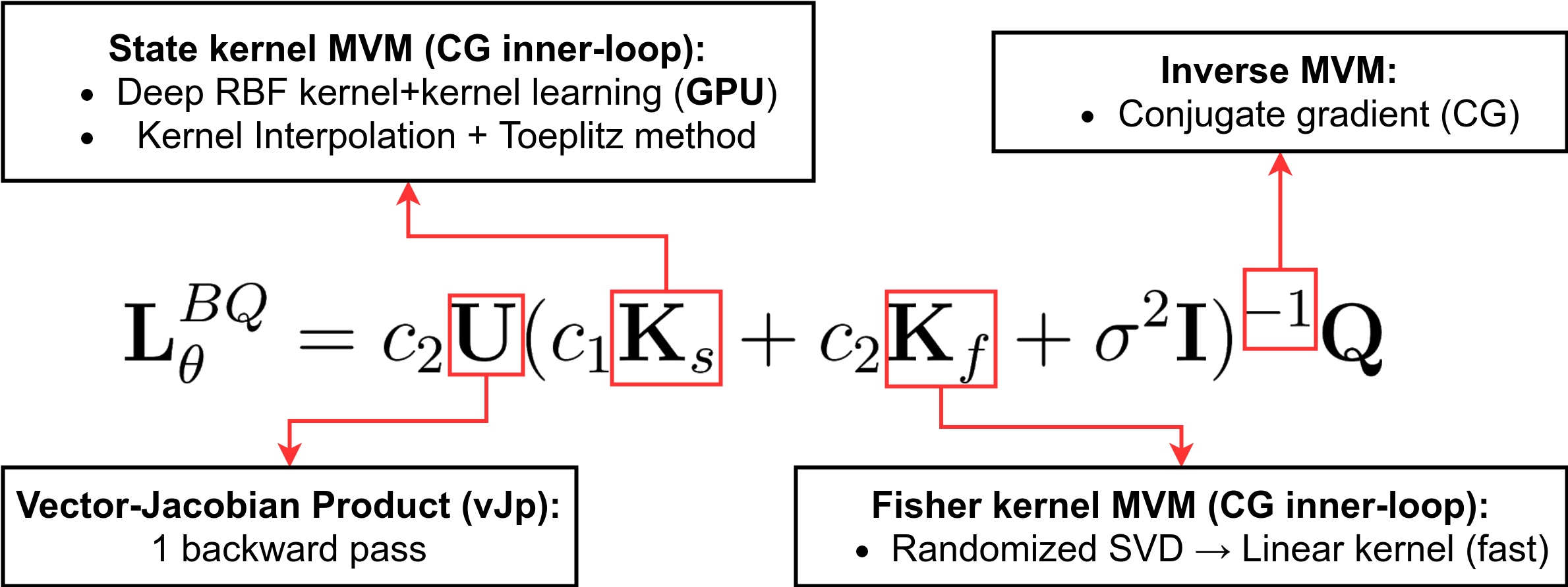
Dealing with Matrix Inversion: First step is to shift the focus from an expensive matrix-inversion operation to an approximate inverse matrix-vector multiplication (i-MVM). In particular, the conjugate gradient (CG) method can be used to compute the i-MVM $(\mathbf{K} +\sigma^2\mathbf{I})^{-1} \mathbf{v}$ within machine precision using $p \ll n$ iterations of MVM operations $\mathbf{K} \mathbf{v}' = c_1 \mathbf{K}_s \mathbf{v}' + c_2 \mathbf{K}_f \mathbf{v}'$. While the CG method nearly reduces the time complexity by an order of $n$, the MVM operation with a dense matrix still incurs a prohibitive $\mathcal{O}(n^2)$ computational cost.

Fast Matrix-Vector Multiplication with $\mathbf{K}_f$: Fortunately, the matrix factorization of $\mathbf{K}_f$ (Eq. \ref{eqn:appendix_kernel_equations}) allows for expressing it as a low-rank linear kernel. All the steps involved in this procedure are linear-time programs based on fast randomized SVD (Halko et al., 2011) and automatic differentiation, without the explicit creation or storage of the $\mathbf{K}_f$ matrix. ← More Details →

Fast Matrix-Vector Multiplication with $\mathbf{K}_s$: Since the choice of state kernel $k_s$ is arbitrary, one can always choose a convenient kernel function that supports fast MVM. Alternatively, one can also approximate the MVM of $\mathbf{K}_s$ using a fast kernel computation method. For instance, structured kernel interpolation (SKI) (Wilson & Nickisch, 2015) is a general kernel sparsification strategy that lowers the computational complexity of $\mathbf{K}_s \mathbf{v}$ MVM from quadratic to linear. ← More Details →

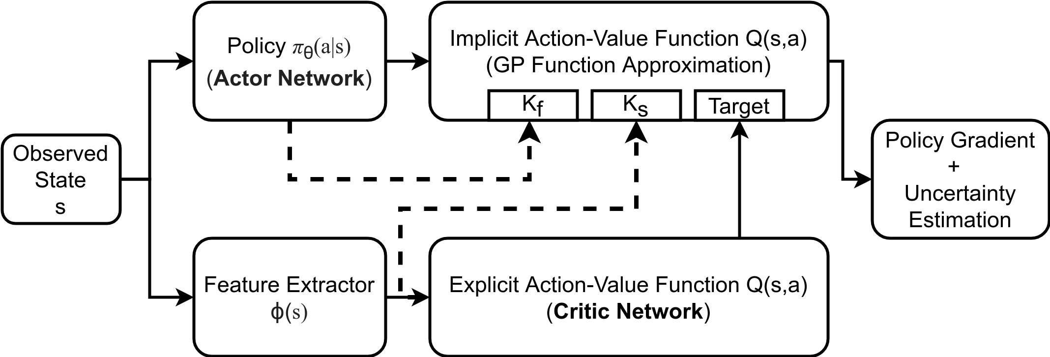
Kernel Learning: As highlighed earlier, BQ-PG can offer more accurate gradient estimates than MC-PG, along with well-calibrated uncertainty estimates, when the state kernel $k_s$ is a better prior that the trivial $k_s = 0$, for modeling the MDP's action-value function $Q_{\pi_{\theta}}$. To make the choice of $k_s$ robust to a diverse range of target MDPs, it is suggested to use a base kernel capable of universal approximation (e.g. RBF kernel), followed by increasing the base kernel's expressive power by using a deep neural network (DNN) to transform its inputs. Deep kernels (Wilson et al., 2016) combine the non-parametric flexibility of GPs with the structural properties of NNs to obtain more expressive kernel functions when compared to their base kernels. The kernel parameters $\phi$ (DNN parameters + base kernel hyperparameters) are tuned using the gradient of GP's negative log marginal likelihood $J_{GP}$ (Rasmussen & Williams, 2005), \begin{align} \label{eqn:GP_nll} J_{GP}(\phi|\mathcal{D}) \propto \log |\mathbf{K}| - \mathbf{Q}^\top \mathbf{K}^{-1} \mathbf{Q}, \quad \nabla_{\phi} J_{GP} = \mathbf{Q}^\top \mathbf{K}^{-1} (\nabla_{\phi}\mathbf{K}) \mathbf{K}^{-1} \mathbf{Q} + Tr(\mathbf{K}^{-1} \nabla_{\phi}\mathbf{K}). \end{align} Practical DBQPG Algorithm: Unlike previous approahces (Ghavamzadeh & Engel, 2007) that compute BQ-PG sequentially, the DBQPG algorithm is designed to directly compute the gradient from a batch of samples (parallelly), thus placing BQ-PG in the context of contemporary PG algorithms. In particular, DBQPG uses a GP to implicitly model the action-value function, and without explicitly constructing the action-value function, returns a Gaussian approximation of the policy gradient, represented by a mean vector (gradient estimate) and covariance (gradient uncertainty). Consequently, this method can also be used with an explicit critic network (different from implicit GP critic) to leverage the orthogonal benefits of actor-critic frameworks (Schulman et al., 2016).

The practical DBQPG implementation is a linear-time program that uses the CG algorithm to deal with the matrix inversion, Fast SVD for Fisher kernel MVM, and SKI for state kernel MVM. Further, the default choice of the state kernel $k_s$ is a deep RBF kernel function, which comprises of an RBF base kernel on top of a DNN feature extractor. The choice of RBF as the base kernel is based on: (i) its compelling theoretical properties such as infinite basis expansion and universal function approximation (Micchelli et al., 2006) and (ii) its compatibility with the Toeplitz method, that provides additional speed-up for SKI computation over stationary kernel. ← More Details →

Uncertainty Aware Policy Gradient (UAPG)

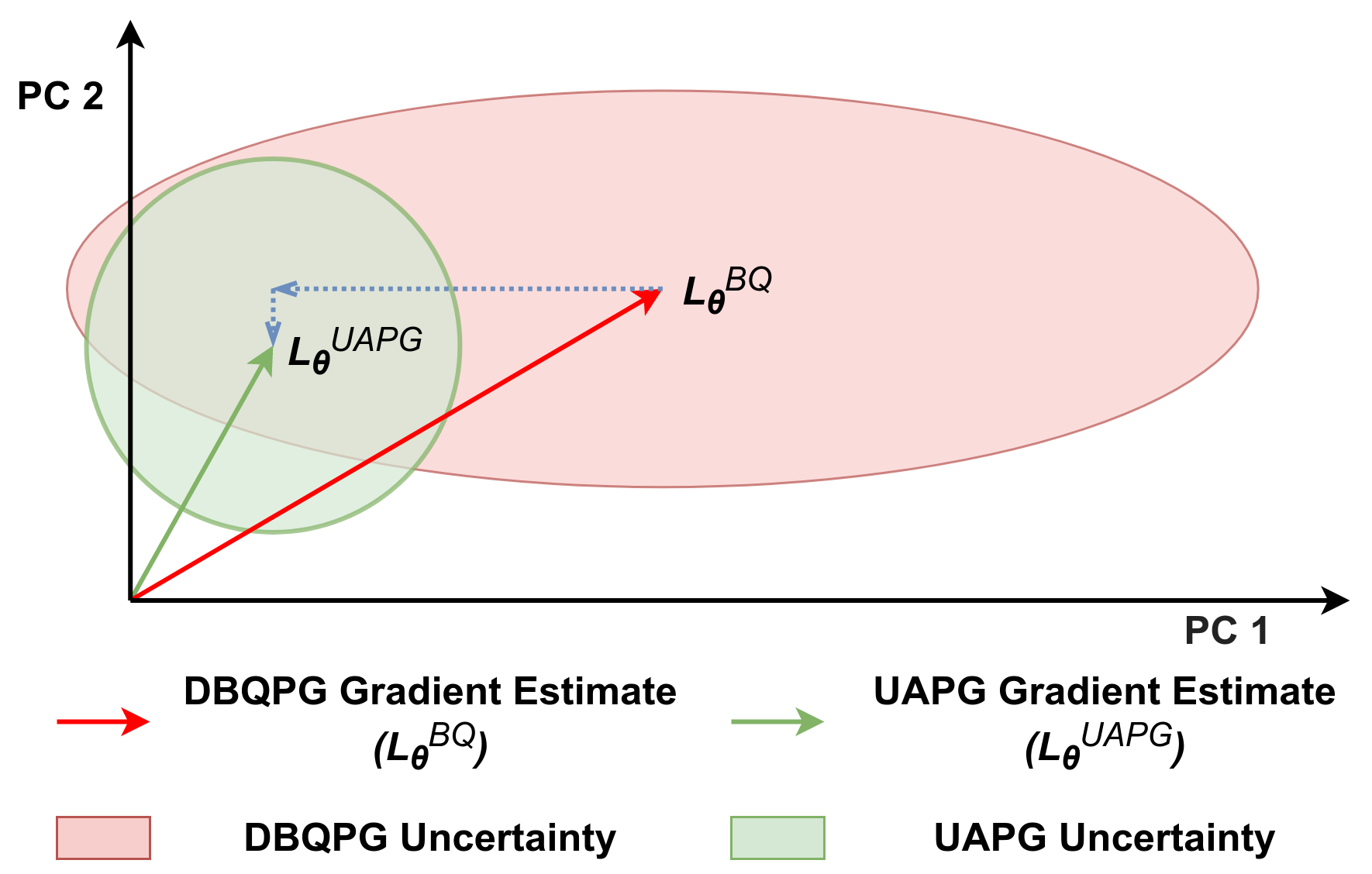
The UAPG method offers more reliable policy updates by utilizing the uncertainty in PG estimation to lower the stepsize along the directions of high gradient uncertainty and vice versa. In particular, the gradient covariance $\mathbf{C}_{\theta}^{BQ}$ from BQ-PG is used to normalize the components of $\mathbf{L}_{\theta}^{BQ}$ with their respective uncertainties, bringing them all to the same scale (uncertainty-wise). Thus, UAPG estimates have uniform uncertainty, i.e. the gradient covariance of the resulting PG estimate is the identity matrix. In theory, the UAPG update can be formulated as \begin{equation} \mathbf{L}_{\theta}^{UAPG} = \big( \mathbf{C}_{\theta}^{BQ} \big)^{-\frac{1}{2}} \mathbf{L}_{\theta}^{BQ}, \qquad \mathbf{C}_{\theta}^{UAPG} = \big( \mathbf{C}_{\theta}^{BQ} \big)^{-\frac{1}{2}} \mathbf{C}_{\theta}^{BQ} \big( \mathbf{C}_{\theta}^{BQ} \big)^{-\frac{1}{2}} = \mathbf{I} \end{equation} Practical UAPG Algorithm: Empirical $\mathbf{C}_{\theta}^{BQ}$ estimates are often ill-conditioned matrices (spectrum decays quickly) with a numerically unstable inversion. Since $\mathbf{C}_{\theta}^{BQ}$ only provides a good estimate of the top few directions of uncertainty, the UAPG update is computed from a rank-$\delta$ singular value decomposition (SVD) approximation of $\mathbf{C}_{\theta}^{BQ} \approx \nu_\delta \mathbf{I} + \sum_{i=1}^{\delta} \mathbf{h}_i (\nu_i - \nu_\delta) \mathbf{h}_i^\top$ as follows: \begin{equation} \label{eqn:UAPG_practical_vanilla} \mathbf{L}_{\theta}^{UAPG} = \nu_{\delta}^{-\frac{1}{2}} \big(\mathbf{I} + \sum\nolimits_{i=1}^{\delta} \mathbf{h}_i \big(\sqrt{{\nu_{\delta}}/{\nu_i}} - \mathbf{I}\big)\mathbf{h}_i^\top \big) \mathbf{L}_{\theta}^{BQ}. \end{equation} The principal components (PCs) $\{\mathbf{h}_i\}_{i=1}^{\delta}$ denote the top $\delta$ directions of uncertainty and the singular values $\{\nu_i\}_{i=1}^{\delta}$ denote their corresponding magnitude of uncertainty. The rank-$\delta$ decomposition of $\mathbf{C}_{\theta}^{BQ}$ can be computed in linear-time using the randomized SVD algorithm (Halko et al., 2011). The UAPG update in Eq. \ref{eqn:UAPG_practical_vanilla} dampens the stepsize of the top $\delta$ directions of uncertainty, relative to the stepsize of remaining gradient components. Thus, in comparison to BQ-PG, UAPG lowers the risk of taking large steps along the directions of high uncertainty, and thereby providing reliable policy updates. ← More Details →

Experimental Results

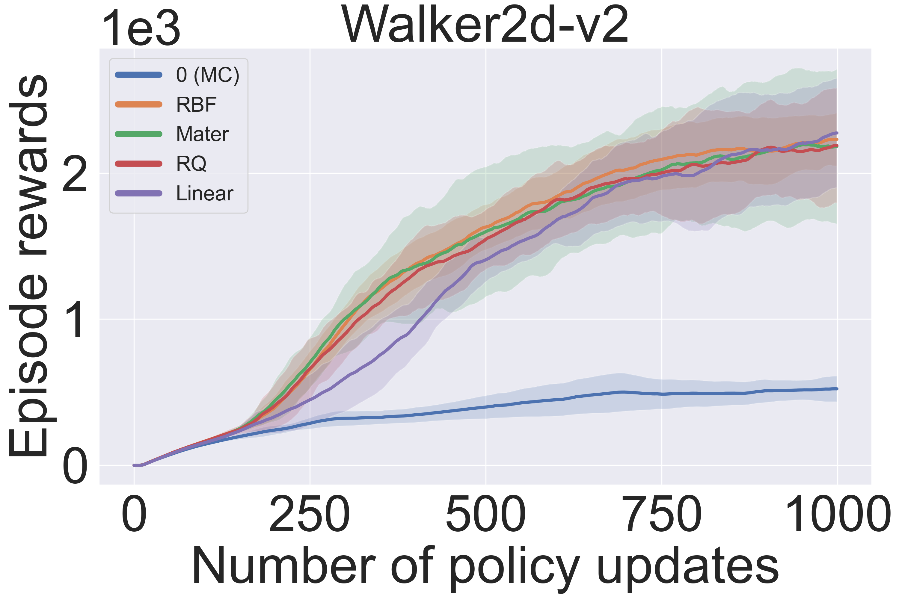
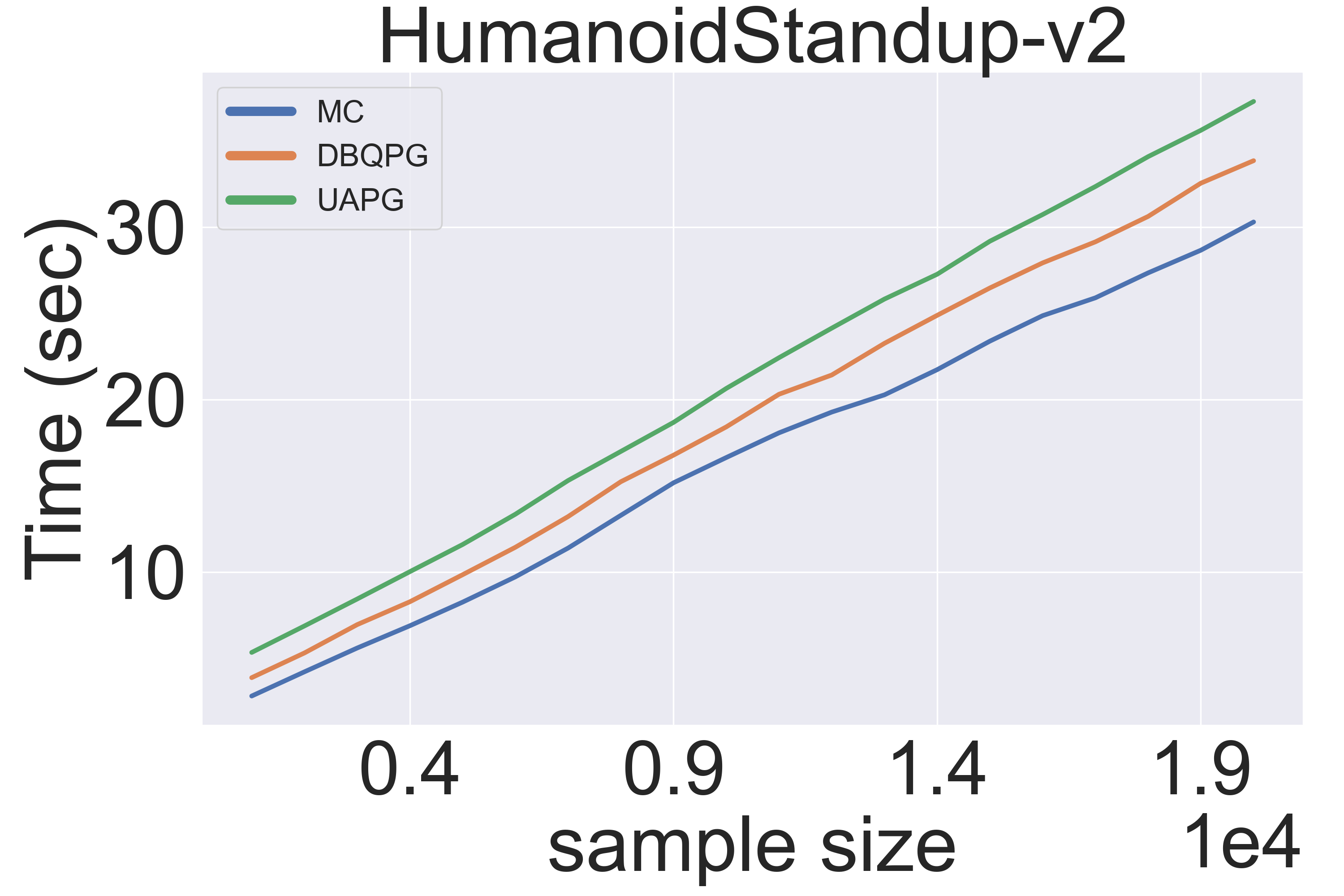
The following observations can be drawn from the first set of experiments (Figure 5):

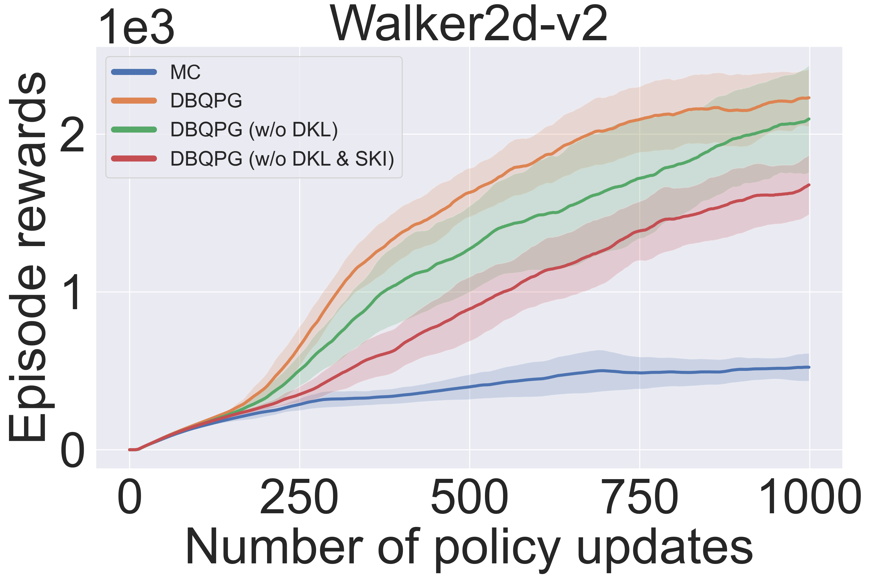
• (Left): deep kernels + kernel learning (DKL) in the state kernel $k_s$ provides better sample complexity and average return when compared to its corresponding base kernel (RBF in this case). Moreover, structured kernel interpolation (SKI) offers better performance relative to traditional inducing point methods, in addition to better computational complexity.
• (Middle): deep kernel learning (DKL) with commonly used base kernels (RBF, Matern, Rational Quadratic, Linear) results in similar performance. This observation provides key insights about the effectiveness of DKL with any (decent) base kernel. More interestingly, all these kernel choices significantly outperform BQ-PG with $k_s = 0$ (equivalent to MC-PG). This highlights the relative inferiority of MC-PG, i.e., BQ-PG with a degenerate prior $k_s = 0$.
• (Right): DBQPG and UAPG methods have a negligible computational overhead over MC-PG, while being significantly more sample efficient, as demonstrated in later experiments. These results were computed on the HumanoidStandup-v2 environment (376-d state and 17-d action space). Also note that the wall-clock time of MC, DBQPG and UAPG methods increases linearly in sample size $n$, which agrees with the complexity analysis in the earlier section.

Quality of Gradient Estimation: Figure 6 compares the quality of PG estimates obtained via DBQPG and MC estimation using two metrics: (i) gradient accuracy or the average cosine similarity of the obtained gradient estimates with respect to the true gradient estimates (estimated from $10^6$ state-action pairs) and (ii) variance in the gradient estimates (normalized by the norm of the mean gradient for scale invariance).

DBQPG clearly provides more accurate gradient estimates with a considerably lower variance than MC estimator. Interestingly, DBQPG and MC estimator offer nearly the same quality gradients at the start of training. However, as the training progresses, and DBQPG learns kernel bases, DBQPG returns superior quality gradient estimates. These results motivate substituting MC with BQ-based gradient estimates in deep PG algorithms.

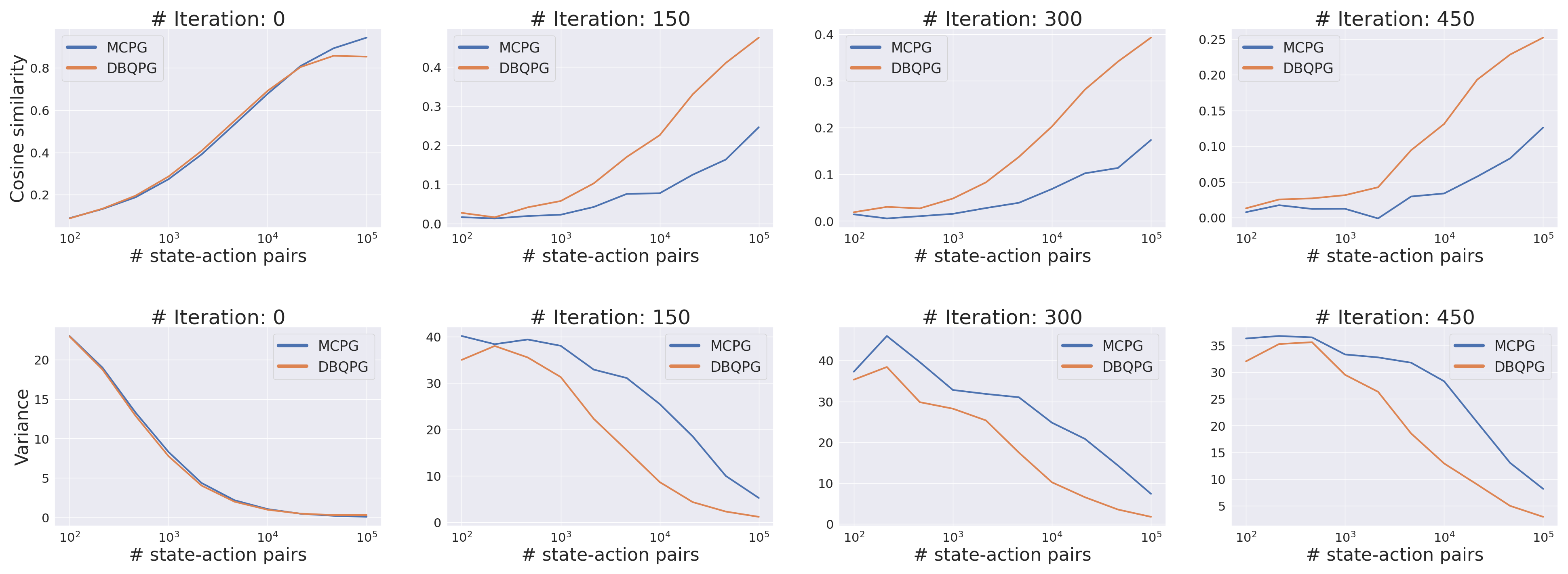
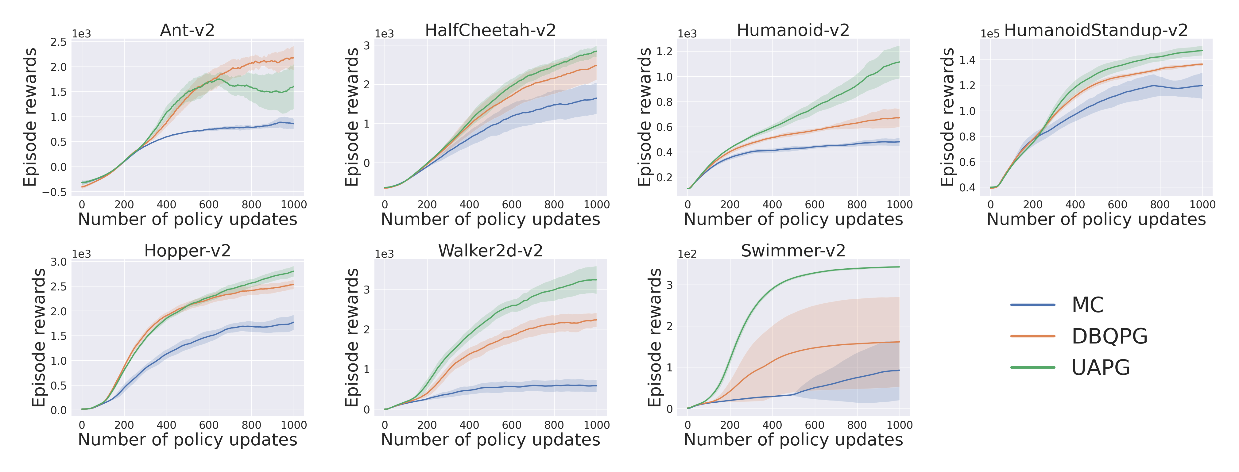
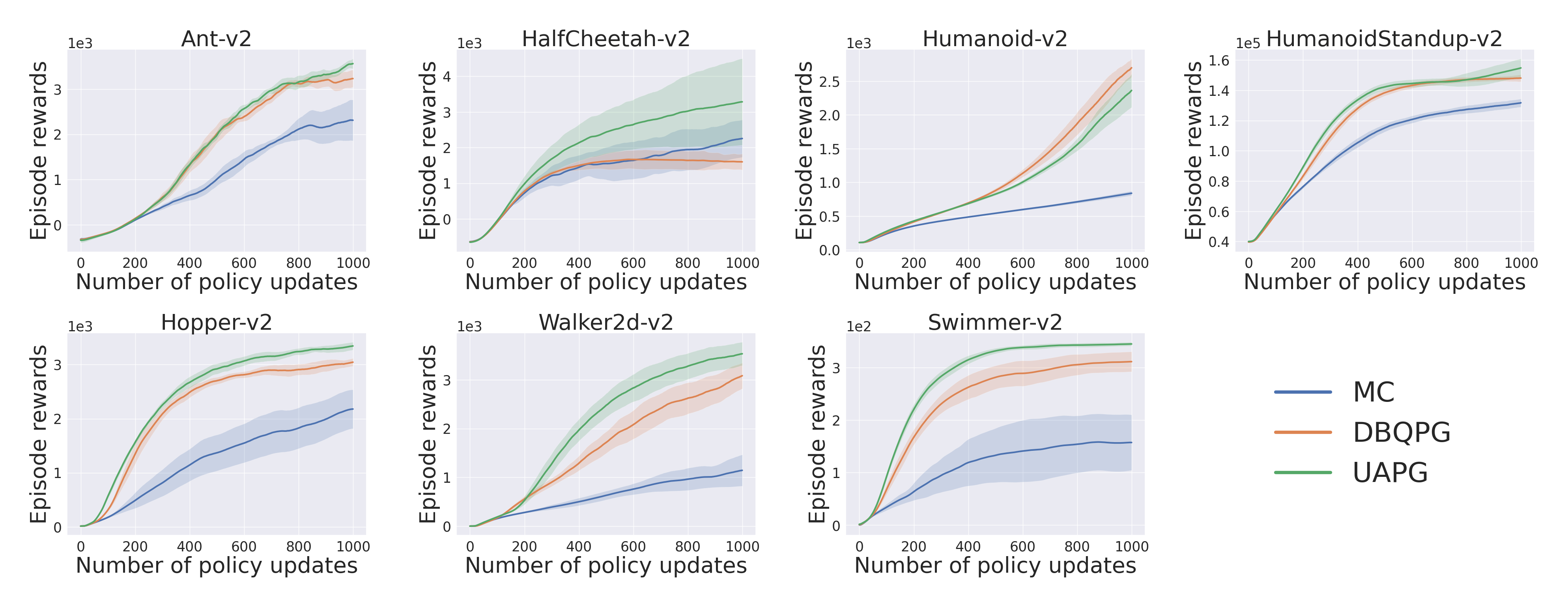
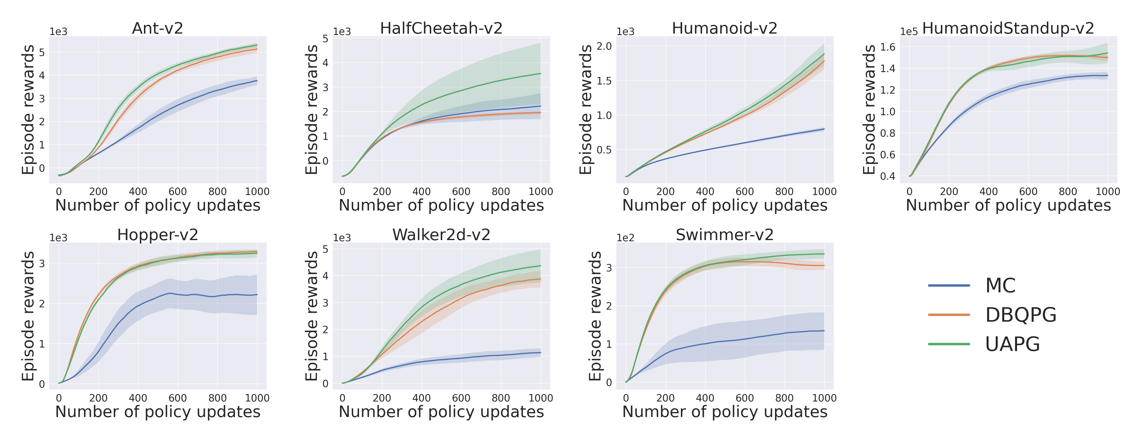
Compatibility with Deep PG Algorithms: Figures 7,8,9 examine the compatibility of DBQPG and UAPG methods with the following on-policy deep policy gradient algorithms: (i) Vanilla policy gradient, (ii) natural policy gradient (NPG), and (iii) trust region policy optimization (TRPO). In these experiments, only the MC estimation subroutine is replaced with BQ-based methods, keeping the rest of the algorithm unchanged. DBQPG consistently outperforms MC estimation, both in final performance and sample complexity across all the deep PG algorithms. This observation resonates with the finding in Figure 6 about the superior gradient quality of DBQPG estimates, and strongly advocates the use of DBQPG over MC for PG estimation.

---

---

The UAPG method performs at least as good as, if not considerably better than, DBQPG on most experiments. The advantage of UAPG estimates is more pronounced in the vanilla PG, and NPG experiments since the performance on these algorithms is highly sensitive to the choice of learning rates. UAPG adjusts the stepsize of each gradient component based on its uncertainty, resulting in a robust update in the face of uncertainty, a better sample complexity, and average return. Since TRPO updates are less sensitive to the learning rate, UAPG adjustment does not provide a significant improvement over DBQPG.

Final Words

In policy gradient (PG) algorithms, the agent estimates the PG using samples gathered through its interaction with the environment, which in real-world is often expensive due to pratical considerations such as time, money or limited resources. Thus, accurate PG estimation from a finite number of samples is a crucial problem in reinforcement learning. However, most contemporary deep PG algorithms use Monte-Carlo (MC) PG estimator, which (i) computes undesirably inaccurate PG estimates with high variance, (ii) suffers from sample inefficiency and a slow convergence rate, and (iii) provides unreliable PG estimates with non-uniform uncertainty which, furthermore, is not explicitly quantified.

Bayesian quadrature (BQ) is a technique for computing accurate policy gradient (PG) estimates from a finite number of samples. DBQPG overcomes the computational challenges of BQ-PG to provide a linear-time routine that can directly substitute MC estimator is contemporary deep PG algorithms. Empirical studies suggest that DBQPG provides more accurate gradient estimates with a significantly lower variance, when compared to MC estimation. Further, replacing the MC estimator with DBQPG in the gradient estimation subroutine of three deep PG algorithms, viz., Vanilla PG, NPG, and TRPO, consistently and considerably improves in the agent's sample complexity and average return. These results strongly advocates the substitution of MC estimator subroutine with DBQPG in deep PG algorithms.

To obtain reliable policy updates from stochastic gradient estimates, one needs to estimate the uncertainty in gradient estimation, in addition to the gradient estimation itself. The UAPG method additionally utilizes the uncertainty in PG estimation quantified by DBQPG, to normalize the gradient components by their uncertainties, returning a uniformly uncertain gradient estimate. Such a normalization will lower the step size of gradient components with high uncertainties and vice versa, resulting in reliable updates with robust step sizes. UAPG uses slightly more computation than DBQPG to provide superior sample complexity and average return. Overall, it is possible to scale Bayesian quadrature to high-dimensional settings, while its better gradient estimation and well-calibrated gradient uncertainty can significantly boost the performance of deep PG algorithms.